Forecast API: time series forecasting with Mistral's Timestral on Opper
By Mattias Lundell -
TL;DR: Send a series' history to POST https://api.opper.ai/v3/forecast with your Opper API key and a model, timestral-5m to timestral-209m, and get back a median and quantiles for every future step. No training, no GPU on your side. Opper runs all four sizes in Stockholm and bills per time step: a day of 15-minute forecasts from three weeks of history costs USD 0.000149 on the largest model. On 28 days of German electricity load every size cut the error of a same-time-last-week forecast by about 40%.
Mistral released Timestral on 15 October 2026: its first time-series foundation models, in four sizes from 5 million to 209 million parameters. You give one a series' history and it returns a probabilistic forecast, zero-shot, with no training on your data. Mistral published the weights and the inference code, and its model page lists no API model id or price. Opper serves all four behind one endpoint.
This post covers the request, a test on four weeks of real grid data (load and day-ahead prices), covariates, what a forecast costs and where it runs.
What Timestral is
- Four sizes, one architecture: 5M, 28M, 123M and 209M parameters. Mistral reports the 209M model first among zero-shot models on GIFT-Eval, TIME and fev-bench, and every size on the accuracy-for-size front.
- Zero-shot: no fine-tuning. Any numeric series with a regular step: demand, sales, sensor readings, traffic, prices.
- Probabilistic: 21 quantiles for every step (0.01, 0.05, 0.1, ..., 0.95, 0.99), so you get a range as well as a number.
- Long history, any horizon: up to 32,768 steps of history; the horizon is decoded in blocks of 1,024 steps.
- More than one variable: several variates forecast jointly, plus past-only, known-future and categorical covariates.
The four sizes on Opper
| Model | Price per 1M input steps | Price per 1M forecast steps | Price of one forecast (2,016 steps to 96) | Time per forecast | Load error, 28 days |
|---|---|---|---|---|---|
| Timestral 5M | USD 0.005 | USD 0.05 | USD 0.0000149 | 0.11 s | 2.45% |
| Timestral 28M | USD 0.01 | USD 0.10 | USD 0.0000298 | 0.21 s | 2.38% |
| Timestral 123M | USD 0.03 | USD 0.30 | USD 0.0000893 | 0.60 s | 2.37% |
| Timestral 209M | USD 0.05 | USD 0.50 | USD 0.000149 | 0.79 s | 2.42% |
The price of one forecast is the history read plus the steps forecast, here three weeks of 15-minute data (2,016 steps) to one day (96 steps). Time is one request with one series, measured end to end over the internet, median of three. Load error is the mean absolute percentage error from the test below.
Model pages, with the same prices and the data-handling facts: 5M, 28M, 123M, 209M. The catalog lists them under the forecast type:
curl -s "https://api.opper.ai/v3/models?type=forecast" \
  | jq -r '.models[] | "\(.id)\tin \(.pricing.input[0])\tout \(.pricing.output[0])"'
Your first forecast
model, prediction_length and series are required. Each series has a target, its history:
curl https://api.opper.ai/v3/forecast \
  -H "Authorization: Bearer $OPPER_API_KEY" \
  -H "Content-Type: application/json" \
  -d '{
    "model": "timestral-209m",
    "prediction_length": 4,
    "series": [{"target": [10, 12, 11, 13, 12, 14, 13, 15, 14, 16, 15, 17]}],
    "quantile_levels": [0.1, 0.5, 0.9]
  }'
{
  "model": "timestral-209m",
  "prediction_length": 4,
  "quantile_levels": [0.1, 0.5, 0.9],
  "forecasts": [{
    "median": [15.92, 17.98, 16.93, 19.07],
    "quantiles": {
      "0.1": [15.63, 17.61, 16.48, 18.48],
      "0.5": [15.92, 17.98, 16.93, 19.07],
      "0.9": [16.28, 18.29, 17.37, 19.58]
    }
  }],
  "usage": {"series": 1, "input_steps": 12, "forecast_steps": 4}
}
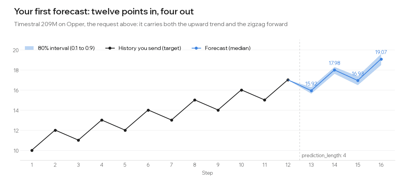
The model picked up both the trend and the up-down zigzag from twelve points. The cost is in the X-Opper-Cost header (here USD 0.0000026), and the call shows up in your traces like any other.
Leave out quantile_levels to get all 21. Two more options default to on, as in Mistral's code: symmetric_averaging (also forecast the negated series and average the two; twice the compute, same price) and clip_nonnegative (keep the forecast at or above zero when the history never goes below it). Turn the second off for a series that can go negative, such as electricity prices.
The same endpoint is on the gateway at https://gw.opper.ai/opper/v1/forecast and https://eu.gw.opper.ai/opper/v1/forecast, with the same body.
A real test: German electricity load
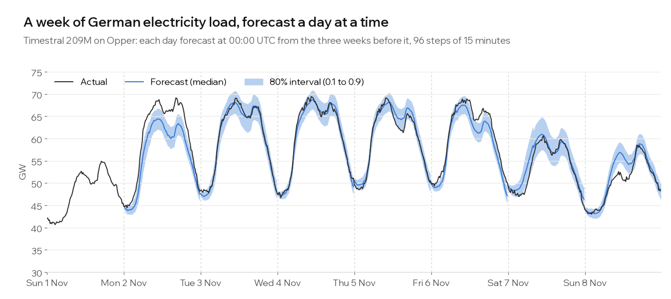
Grid load is the case Mistral's announcement uses: one day ahead, from three weeks of 15-minute history. We took Germany's measured load from Energy-Charts by Fraunhofer ISE and forecast each of the 28 days from 12 October to 8 November 2026 at 00:00 UTC, from the 2,016 steps before it. Every size got the same 28 histories, seven series to a request. The baseline is the usual naive forecast for load: the same 15 minutes one week earlier.
| Forecast | Mean absolute error | Mean absolute % error | Actuals inside the 80% interval |
|---|---|---|---|
| Same 15 minutes last week | 2.26 GW | 4.07% | n/a |
| Timestral 5M | 1.38 GW | 2.45% | 84.0% |
| Timestral 28M | 1.33 GW | 2.38% | 82.6% |
| Timestral 123M | 1.33 GW | 2.37% | 80.6% |
| Timestral 209M | 1.35 GW | 2.42% | 78.8% |
What the numbers say:
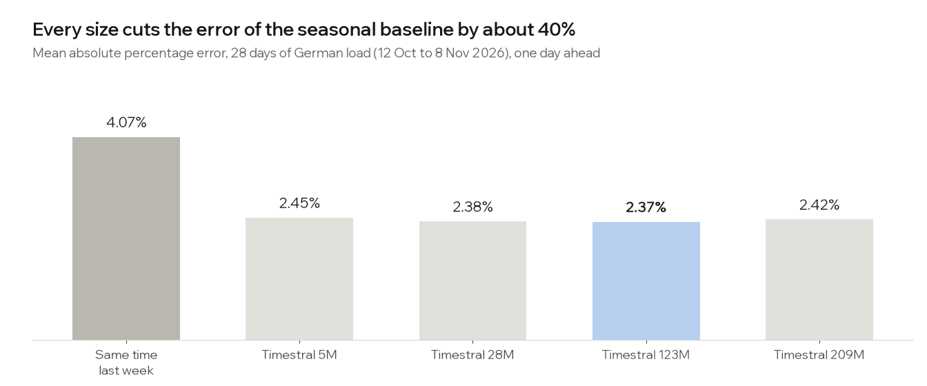
- Every size cut the baseline's error by about 40%, from 4.07% to between 2.37% and 2.45%, on a series averaging 55 GW. 209M beat the baseline on 26 of the 28 days.
- The sizes were within 0.08 percentage points of each other. 123M was best and 5M last, at a sixth of 123M's price and a fifth of its time. Mistral's benchmarks rank 209M first over many datasets; on one clean, strongly seasonal series like national load, the small models already find what there is to find.
- The intervals are honest: 79% to 84% of actual values fell inside the 80% interval, and the 0.9 quantile was above the actual load 87% to 91% of the time. That is what makes a quantile usable for planning capacity.
- The worst day was Monday 2 November (5.9% on 209M, and one of the baseline's worst days too), with the forecast low through the working day. Calendar effects such as public holidays and school breaks are not in a series' history unless you pass them as covariates.
Known covariates: day-ahead prices with wind and solar
Prices are harder. The German day-ahead price swings with wind and solar output, which the price's own history cannot see coming. That is what known covariates are for: rows you pass for the history and the forecast window both, such as a weather forecast, a promotion calendar or holidays.
Each covariate row is as long as the target plus prediction_length:
{
  "model": "timestral-209m",
  "prediction_length": 96,
  "clip_nonnegative": false,
  "series": [{
    "target": [/* 2,016 prices, EUR/MWh */],
    "known_covariates": [
      [/* wind, 2,016 + 96 values */],
      [/* solar, 2,016 + 96 values */],
      [/* load, 2,016 + 96 values */]
    ]
  }]
}
Same 28 days, the German-Luxembourg (DE-LU) day-ahead price as the target, from SMARD.de (Bundesnetzagentur, CC BY 4.0) through Energy-Charts:
| Forecast | Mean absolute error (EUR/MWh) | Actuals inside the 80% interval |
|---|---|---|
| Same 15 minutes yesterday | 40.7 | n/a |
| Same 15 minutes last week | 84.0 | n/a |
| Timestral 28M, price history only | 27.4 | 82.4% |
| Timestral 209M, price history only | 27.1 | 81.2% |
| Timestral 28M, with wind, solar and load | 19.4 | 80.2% |
| Timestral 209M, with wind, solar and load | 17.7 | 79.3% |
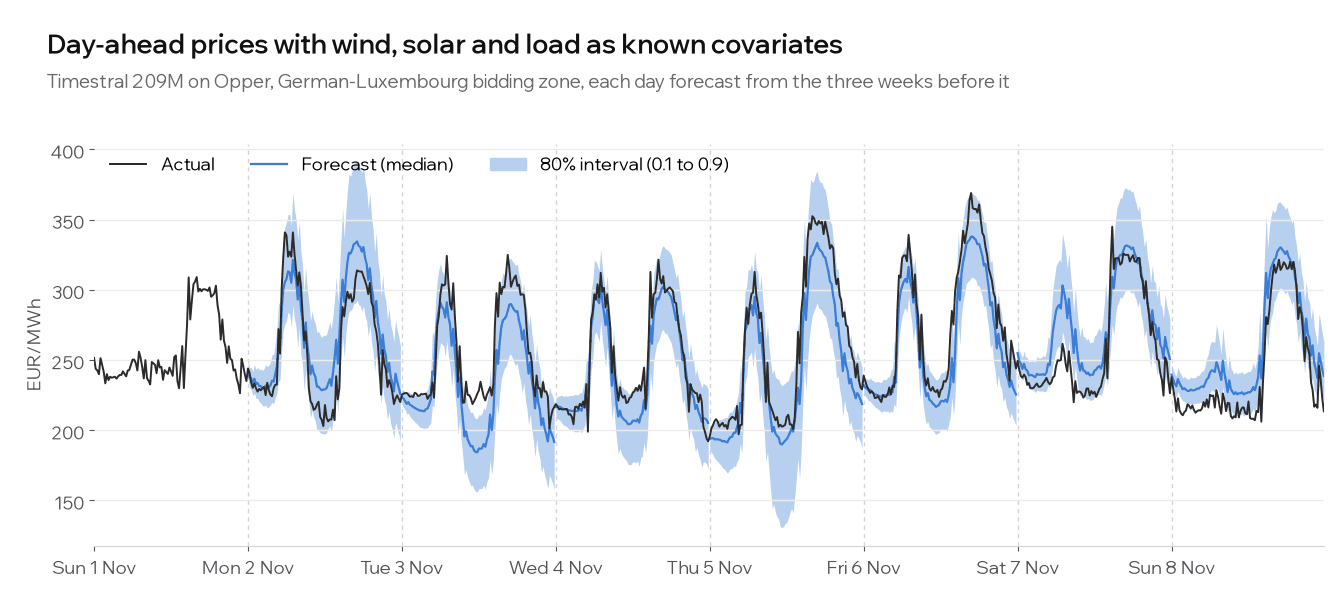
Prices over the 28 days averaged EUR 201/MWh and ranged from zero to EUR 574/MWh, which is why there is no percentage column: a percentage error is meaningless around zero.
- From its own history, Timestral cut the error of "same as yesterday" by a third (40.7 to 27.1 EUR/MWh).
- Wind, solar and load cut it by another third (27.1 to 17.7 on 209M, 27.4 to 19.4 on 28M), and on 209M covariates won on 20 of the 28 days.
- The bigger model used the covariates better: without them 28M and 209M were 0.3 EUR/MWh apart, with them 1.7.
- Covariates make a request heavier: four rows are read instead of one, so input cost is four times higher, and a request of seven series took about 32 seconds on 209M instead of 5.
One caveat on that row: we passed the measured wind, solar and load for the forecast day, where in production you would pass their forecasts. A weather forecast is less exact than the measurement, so read the covariate result as the most covariates can add here.
Past covariates (past_covariates, as long as the target) are for series you only know up to now, and the categorical variants take category codes, such as a store id or a weekday, and are target-encoded per series.
Many series, several variates, missing values
- Many series in one request: put up to 1,024 in
series, and they are forecast together. Series of different lengths are padded to the longest. - Several variates jointly: make
targeta list of equally long lists, such as the load of three regions, and the forecast keeps the same shape, so the model can use how they move together. - Missing values:
nullanywhere in a target or a covariate row.
What it costs
Opper bills per time step, from the response's usage: every step read (each target variate and each covariate row) at the input price, every step forecast at the forecast price. Nothing else, no per-request fee.
- One day of 15-minute load from three weeks of history (2,016 read, 96 forecast) on 209M: USD 0.000149. A million such forecasts: USD 148.80.
- The same on 5M: USD 0.0000149, or USD 14.88 per million.
- With three known covariates, a request reads four rows instead of one, so its input cost is four times higher.
The whole 28-day test above, every model and both targets, cost under 3 US cents (USD 0.029).
Where it runs and what is kept
Opper runs all four models itself, in AWS's Stockholm region (eu-north-1), so a series stays in the EU and passes through no model provider on the way. The forecasting service stores nothing and logs only the shape of each request (how many series and steps), never the numbers. Opper's own record of the call, which you see in your traces (if enabled), follows your organization's retention setting, and at zero nothing is kept. An organization rule that allows only EU inference or zero data retention lets these calls through.
Limits
- Up to 32,768 steps of history per series are read; longer histories keep the most recent.
- Up to 8,192 steps of horizon, 1,024 series, about 4 million numbers and 64 MiB per request.
- Bigger requests take longer: in the test, a request of seven series with three covariate rows each took about 32 seconds on 209M. A
503means every forecast slot is taken; retry shortly. - A forecast is only as good as the history: a regime change the history never showed, such as a new tariff or a plant going offline, is invisible to the model unless you pass it as a covariate.
Which size to pick
- Start with 28M. It was within 0.01 percentage points of the best on load, costs a fifth of 209M and answers a single series in about 0.2 seconds.
- Pick 5M for very many series or a tight latency budget: about 0.1 seconds and USD 14.88 per million day-ahead forecasts of the shape above, at 0.08 points behind on load.
- Pick 209M when you pass covariates or your series are noisier than national load. It gained the most from covariates in the price test, and it is the size that ranks first in Mistral's benchmarks.
- Test on your own history first. Hold back the last few days, forecast them from what came before, and compare. It is the same request, and the 28-day test above cost under 3 cents.
Get started
- Opper platform →: get an API key and send your first forecast.
- Timestral 209M on Opper →: prices, region and data handling for each size.
- Mistral's Timestral announcement →: the architecture and the benchmark results.